Loudspeaker Impedance – A Designer’s View by Phil Jones

Loudspeaker Impedance – A Designer’s View

Phil Jones – speaker designer

 

Abstract

Most players think of a speaker as a simple “4 ohm” or “8 ohm” load that turns watts into noise. From the designer’s chair it looks very different. Impedance is not a single number, it is a moving target that changes with frequency, cone position, temperature, magnet behaviour and even the recent history of the last few notes you played. This paper is my attempt to pull all of those pieces together in one place and explain what is really going on at the terminals of a loudspeaker, and what that means for tone, reliability and cabinet design. I will keep the maths as friendly as possible but not shy away from it where it really helps to tell the story.

1. Introduction – the “room heater” view of a loudspeaker

When I look at a bass cabinet I do not see a musical instrument first. I see a very efficient electrical heater that happens to make sound as a side effect. A typical bass box might turn only one or two percent of the electrical power it swallows into acoustic power. The rest becomes heat in the voice coil, the magnet structure and the air trapped inside the box. At high power the voice coil can be running at more than two hundred degrees Celsius while you are standing a few metres away enjoying the groove. Because almost all of the input power becomes heat, the electrical impedance of the driver is not a constant. The dc resistance of the coil rises nwith temperature, the inductance changes as the magnetic circuit is pushed around by the signal and the mechanical system shifts as the suspension and air load heat up. On top of that, the cone motion feeds a voltage back into the amplifier – back electromotive force, or back EMF – so the driver
acts as a generator as much as it does as a load.

 

If you only ever looked at the nominal impedance on the spec sheet you would miss almost all of this. The job of a designer is to understand how impedance moves in the real world and to bend that behaviour towards musical goals: more headroom, less distortion, better dynamics and predictable power handling.

2. What loudspeaker impedance really is

Impedance is the AC cousin of resistance. In a pure resistor the current and voltage are in step and the power is simply P = V × I. A loudspeaker is not a pure resistor. The voice coil has resistance, the winding behaves as an binductor and the moving system stores and releases mechanical energy just like a mass on a spring. If we write the impedance as a complex number we have Z(ω) = R(ω) + j X(ω) where R(ω) is the resistive part, X(ω) is the reactive part and ω = 2πf is the angular frequency. The magnitude of the impedance is |Z| = √(R² + X²) and the phase angle is φ = arctan(X / R). The useful electrical power that actually heats the coil is P = V × I × cos φ When the phase angle is large the amplifier is supplying a lot of current that is merely shuttling energy in and out of the mechanical system rather than heating the voice coil. Around resonance, for example, the apparent impedance of the driver can be very high – perhaps thirty ohms – even though the dc resistance of the coil might only be six or seven ohms. So when we talk about a “4 ohm” or “8 ohm” speaker we are really talking about the approximate mid‑band magnitude of |Z| where the driver behaves mostly resistively. Away from that region the curve moves all over the place, and that movement is where the interesting physics lives.

3. The classic four‑part impedance curve

Every moving‑coil loudspeaker shows the same basic impedance fingerprint when you sweep it from the deep bass to the top of its useful range. It is convenient to think of this curve in four regions.

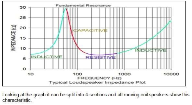
Figure 1 – Typical loudspeaker impedance curve with the four regions
labelled.

Starting at very low frequency, below the driver’s free‑air resonance, the suspension acts like a spring whose reactance rises as the frequency falls. In this region the impedance has an inductive character because the cone is almost locked in place by the stiffness of the surround and spider. As we approach mechanical resonance the mass of the moving system and the stiffness of the suspension exchange energy like a mass bouncing on a spring. The impedance shoots up to a sharp peak, often four or five times the nominal mid‑band value. This is the “fundamental resonance” that everybody recognises. The exact height and sharpness of this peak are controlled by the mechanical losses in the suspension and the electrical damping from the amplifier.

Above resonance the curve drops into a broad trough where the driver looks mostly resistive. This is the region where most of the useful bass andlow‑mid energy of a woofer lives. The impedance here is not perfectly flat – box loading, leakage and damping all put their fingerprints on it – but it is close enough to the nominal rating that an amplifier designer can treat it as Ohm’s law territory.

At higher frequencies the inductance of the voice coil dominates and the impedance rises again with a gentle slope. This is the part of the curve that many people glance at and then forget, but as we will see, the way that inductance behaves with frequency, cone position and temperature has a huge effect on distortion and tone.

4. Box loading and the low‑frequency impedance

Mounting the driver in a cabinet reshapes the low‑frequency part of the impedance curve. A sealed box adds an air spring in parallel with the suspension. The resonance frequency rises and the single peak on the impedance curve broadens and lowers a little. A vented (bass‑reflex) box is more dramatic: the air in the port and the air in the box form a tuned resonator that adds a second peak to the impedance curve. Between those two peaks sits the tuning frequency where the cone motion is at a minimum and the port does most of the work.

 

A horn‑loaded system goes even further by presenting the cone with a highly resistive air load over its pass band. The impedance curve develops multiple peaks and dips that reflect the horn’s own resonances and cut‑off frequency. From the amplifier’s point of view these systems are all just different complex loads, but from the player’s point of view they feel very different. The way the cone is allowed to move or held back at low frequencies determines not only the tonal  alance but also how much thermal and mechanical stress the driver sees for a given SPL.

5. Modelling the voice‑coil inductance

At mid and high frequencies the dominant part of the impedance is the voice‑coil inductance and the losses associated with it. The simple textbook model is a resistance Re in series with an ideal inductance Le. That is good enough for school physics, but it completely ignores the real magnetic circuit: steel pole pieces, top plate, magnet, shorting rings and the conductive former. All of these parts support eddy currents that fight against changes in flux and add a lossy, frequency‑dependent term to the impedance.

A useful way to capture this behaviour is the so‑called LR‑2 model. The excess impedance of the voice coil (with the motional part and dc resistance removed) is represented as Z_L(jω, x) = j ω L_e(x) + [ R_2(x) · j ω L_2(x) ] / [ R_2(x) + j ω L_2(x) ] Here L_e(x) is a series inductance, and L_2(x) in parallel with R_2(x) represents the eddy‑current path in the surrounding metal. All three parameters depend on cone displacement x because moving the coil in and out of the gap changes how tightly it couples to the steel and to any shorting rings or copper caps. For design work it is useful to write these parameters as power‑series in displacement, for example L_e(x) = l₀ + l₁ x + l₂ x² + …and similarly for L₂(x) and R₂(x). The coefficients describe how quickly inductance and loss change as the coil moves. If those curves are symmetrical about x = 0 the resulting distortion is dominated by odd order components. Any asymmetry – very common when a shorting ring is only on one side of the gap – produces strong second‑order and other even‑order distortion.

6. Suspension stiffness and its impact on impedance

The suspension – surround, spider and even the cone itself – is not a linear spring. The restoring force is better described as F = K(x) · x, where the stiffness K(x) increases as the cone approaches the limits of its travel. In extreme cases K(x) may change by a factor of twenty or more between rest and full excursion.

One way to see this is to clamp a suspension in a sealed box, drive it pneumatically and measure its displacement and the air pressure that is moving it. From those two signals we can estimate K(x) over the full travel using system‑identification techniques. If we plot K(x) against x we usually see two important features. First, the curve is strongly level‑dependent: at small excursions around the origin it is almost flat, but at larger excursions it rises steeply. Second, the curve is often not symmetrical. The stiffness for positive displacement can be very different from that for negative displacement. This non‑linear stiffness feeds directly into the impedance peak at resonance. The effective stiffness K_eff depends on the peak displacement X_peak, and the resonance frequency follows ω_R² = K_eff(X_peak) / m where m is the moving mass. As you turn up the volume and the cone swings further, K_eff rises, ω_R moves upwards and the shape of the
impedance peak changes. An asymmetric K(x) also generates a dc shift of the rest position under large signals, which moves the coil awmagnetic centre of the gap and interacts with the inductance nonlinearity described earlier.

7. Temperature, resistance and power compression

The voice coil is where nearly all of the electrical input power ends up. The resistance of the wire increases with temperature according to R_e(T) ≈ R_e(T₀) · [ 1 + α · (T − T₀) ] where α is the temperature coefficient of resistance. For copper it is typically about 0.004 per degree Celsius, roughly a 0.4 % increase in resistance for every degree the coil heats above ambient. Aluminium is roughly half of that, around 0.0026–0.0028 per degree, which is one reason why copper‑clad aluminium wire is so attractive for high‑performance drivers: it lets us pack a lot of conductor into the gap with less mass and less change of resistance as the coil cooks. Suppose an 8 ohm coil made from copper wire rises by 150 °C during a long loud passage. With α = 0.004 the hot resistance is R_hot ≈ 8 · [ 1 + 0.004 × 150 ] ≈ 8 · 1.6 ≈ 12.8 Ω

From the amplifier’s point of view the load has quietly drifted from 8 ohms to nearly 13 ohms. If the amp is a near‑ideal voltage source the current drops in proportion and the acoustic output falls by several decibels even though you have not touched the volume control. This is thermal power compression.

The problem does not stop at the voice coil. As the steel and magnet heat up, their magnetic properties change. The available flux in the gap falls, the BL product drops and the driver loses sensitivity. In many real cabinets the thermal time constant of the motor is several minutes, so a hard‑driven rig can lose punch over the first song and stay slightly “sleepy” until it has time to cool.8. Back EMF, flux modulation and strong transients

Any time a conductor moves in a magnetic field it generates a voltage. In a loudspeaker this back EMF is e = B · l · v = Bl · v where B is the flux density in the gap, l is the length of wire in the field and v is cone velocity. In the equivalent circuit this appears as a voltage source in series with the voice coil. Around resonance the back EMF can dominate the electrical behaviour: the driver actually tries to drive current back into the amplifier. That is why the impedance peak at  esonance can be so high m– the mechanical system is feeding energy back instead of absorbing it. Under high‑power transients the current in the voice coil becomes large enough that its own field is no longer a small perturbation on top of the permanent magnet’s field. The coil field either adds to or subtracts from the steady field depending on the instantaneous current direction. In the steel parts this can bend the flux lines, push regions of the pole piece towards saturation and, in extreme cases, reduce the effective field in the gap during the peaks of the waveform.

From the impedance point of view this flux modulation shows up as a time‑varying BL product and a time‑varying inductance. As the field is reduced, Le and BL fall, so the impedance at mid and high frequencies drops and the current spikes even harder. Certain magnet materials are also vulnerable to demagnetisation if the opposing field from the coil is large enough and long enough. Modern magnets are much better behaved than those from decades ago, but when you design for very high peak current you still have to look carefully at the B–H curves of the chosen materials.

9. Dynamic impedance under real programme material

Real music is not a steady sine wave. A loud bass transient might last only a few cycles. At the startsmall‑signal value and the suspension is close to linear. The instantaneous impedance is therefore at its “fresh” value and the current can be very high. As the note continues, the coil heats, Re rises, the suspension stiffens slightly with excursion and the magnet structure warms up. The impedance seen by the amplifier is a moving target with thermal time constants ranging  from tens of milliseconds to many seconds.If the programme consists of repeated high‑crest‑factor bursts – typical of slap bass or kick‑drum‑heavy material – the driver never really returns to its cold state. Each burst starts from a hotter baseline than the previous one, so the dynamics are compressed in a very subtle way. Players experience this as a cabinet that feels punchy and responsive at the start of the set but slightly “squashed” later on when everything is hot. Good thermal design and sensible impedance behaviour minimise this effect but they never erase it – it is built into the physics of moving‑coil speakers.

10. Amplifier source impedance and damping factor

No discussion of loudspeaker impedance is complete without touching on the amplifier. A real amplifier has some finite output impedance R_g. The ratio of load impedance to source impedance is the damping factor. From the loudspeaker’s point of view what matters is the total series resistance between the voice coil and the voltage source: amplifier output, speaker cable, connectors and any series components in the crossover. For a closed‑box system the electrical losses appear in the total Q of the system. A convenient expression is Q_tc = Q_tco · ( R_e + R_g ) / R_e where Q_tco is the system Q with zero source resistance. A little added resistance raises Q_tc, making the bass slightly looser and more emphasised around resonance. In practice the resistance of the cable and the inductor in a passive crossover often dominates once the amplifier’s damping factor is higher than aboutamplifier specifications brings rapidly diminishing returns unless the rest of the system is carefully engineered to take advantage of them.

11. Measuring impedance in the workshop

It is perfectly possible to learn a great deal about a driver with basic test gear. One simple method is to turn a sine‑wave generator into a near‑constant‑current source using a large series resistor – say 1 kΩ – and then measure the small voltage across the loudspeaker as you sweep frequency. If you adjust the generator so that a known calibration resistor reads, for example, 8 mV, that corresponds to 1 mA of test current, and the mV reading on the meter is numerically equal to the impedance in Ohms. By finding the frequency of the main impedance peak and the frequencies on either side where the impedance falls to a defined fraction of that peak, you can calculate the mechanical and electrical Q values of the driver and its free‑air resonance. Adding a known mass to the cone and repeating the measurement lets you estimate the compliance and equivalent volume of air (Vas). Modern analyser systems do all of this automatically and can also sweep displacement and temperature, but it is still instructive to go through the process by hand at least once.

12. Design strategies for civilised impedance behaviour

Once you accept that impedance is not a fixed number but a whole landscape, loudspeaker design becomes a game of sculpting that landscape.

A few key strategies help:

• Use large, well‑ventilated voice coils and, where appropriate, copper‑clad aluminium windings to reduce mass and thermal compression.

• Shape the magnetic circuit with shorting rings, copper caps and carefully chosen steel geometry so that Le(x) and Re(f, x) are as flat and symmetric as possible over the working stroke.• Design the suspension so that K(x) stays reasonably soft over the intended excursion range and avoids sharp asymmetries that would push the coil off‑centre under drive.

• Choose box alignments that control cone excursion where it is most dangerous without presenting wild swings of impedance that could upset the amplifier.

• Think about thermal paths from the coil to the outside world – vents, aluminium formers, heatsinking to the magnet – so that the inevitable heat is moved away quickly.

None of these tricks changes the underlying laws of physics. You cannot get deep bass, small size and high efficiency all at the same time; you can only trade between them. But by managing the impedance in a sensible way you can decide exactly where those trade‑offs land and how the system behaves when it is pushed hard on stage.

13. Closing thoughts

From the outside a loudspeaker looks simple – a cone, a dustcap and a magnet. From the terminals looking in it is anything but simple. The impedance that the amplifier sees is a living, breathing thing that moves with frequency, displacement, temperature and time. Understanding that behaviour is the key to building cabinets that stay musical when they are working hard, that survive the abuse players throw at them, and that translate every nuance of the instrument instead of ironing it flat. My hope is that this overview gives you a feel for what is going on under the hood. The next time you look at an impedance curve, or feel your rig start to soften up after a long set, you will know that you are really hearing the physics of impedance changing in real time – and that, as a designer, I have spent a large part of my life trying to make those changes work in your favour rather than against you.